We left off from the last post after performing an ANOVA statistical test and showing that there is a difference between treatments. Our next steps are to build a model and then check our model and assumptions we had previously made are correct.

Outline

• Model the data
• Computing residuals
• Testing assumptions with residuals
• Check for outliers

Model the data

At this stage, we have enough information to build a simple model. Remember from Part I that we were using an effects model with a single factor or treatment. The skeleton for this model is:

We can simplify $\mu$ and $\tau_{i}$ by taking $\mu_{i}= \mu + \tau_{i}$

From my previous post we had created a dataframe, yi_avg, which was the average under the i-th treatment. It turns out that this average is also a good estimate for our point estimator, $\hat{y}_{i}$. Tip: Anything you see with a hat over a variable means that it is an estimator. We can now create our model:

y_hat = yi_avg.copy()
y_hat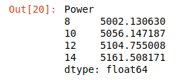

Great! Now we have a simple model using Power to predict our outcome variable, y (CVD growth rate).

Computing residuals

To calculate our residuals, we need to subtract our model from our actual values:

cvd_pivot_residuals = cvd_pivot.sub(y_hat, axis = 1)
cvd_pivot_residuals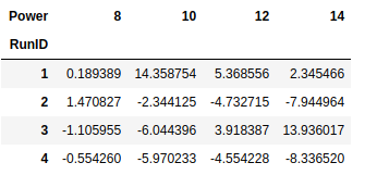

And melt them back into a singular column for analysis with Python.

cvd_pivot_residuals_melted = cvd_pivot_residuals.melt()
cvd_pivot_residuals_melted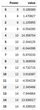

Testing assumptions with residuals

From here we need to check the assumptions we originally made. We do that by:

• Checking normality against residuals,
• Plot versus time sequence,
• Plot versus fitted values, and
• Checking for outliers

One of the first assumptions we made when running an ANOVA was that the data was approximately normal. We typically check this with a histogram but because we have a small sample set, small fluctuations in our data causes large shape changes to our histogram. Instead we check our residuals with a normal probability plot. What we are interested in from our probability plot is whether our residuals are approximately normal.

from scipy import stats
stats.probplot(cvd_pivot_residuals_melted['value'], plot=plt)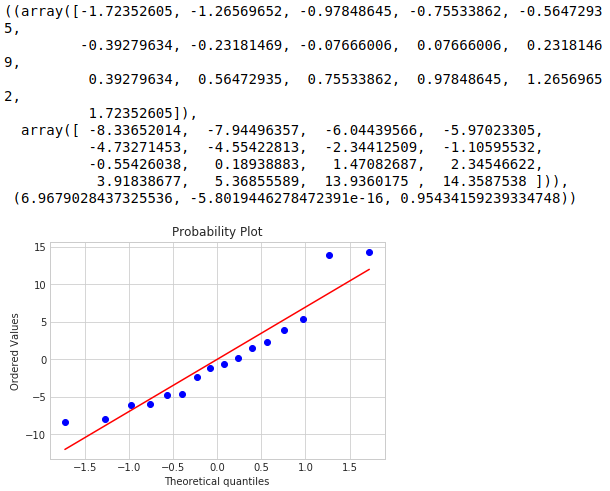

The most important thing here is if the data between the -1 and +1 quantiles are approximately linear. From the probability plot we see that our data is approximately linear with some deviations on the tails.

At this point we would check to see if there is correlation between samples run in time sequence. If there was, then our assumption of independence between runs is false. Unfortunately since I created this data set, we will not be calculating it here.

The next check is to make sure that there is consistent variance between treatments. An unequal variance can cause deviations in our F-Test but will mainly affect experiments with unequal treatment sizes or a different type of model.

To set this up we have to reset our power settings to our power average value.

for power_setting, power_avg in mu_hat.iteritems():
    cvd_pivot_residuals_melted.loc[cvd_pivot_residuals_melted['Power'] == power_setting, 'Power'] = power_avg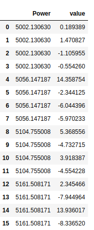

plt.scatter(cvd_pivot_residuals_melted['Power'], cvd_pivot_residuals_melted['value'])
plt.xlabel('Predicted Growth Rate')
plt.ylabel('Residuals')
plt.show()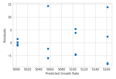

So with this chart we see that there are some differences in variance. With our balanced designed (same number of samples per treatment) this does not cause a large effect on our F-test. An important point here is that the last few tests showed some deviations from normality and a deviation from homogeneous variance. We were able to continue with our test because of our balanced experiment. Having a balanced experiment helps minimize deviations so we can accurately interpret the experiment.

Check for outliers

Looking at our data in the predicted vs. residual chart we see some large deviations from set to set. Lets check and see if they are outliers. A simple check is by checking the standardized residuals:

where $e_{ij}$ is our residual, and $MSE$ is our mean squared error calculated previously. This equation normalizes our residuals and most of the data (~95%) should fall within $\pm$2 from our mean. Anything greater than 3 is a potential outlier.

def check_outliers(residuals, mean_square_error):
    check_out = residuals.iloc[:,1:].divide(mean_square_error ** (0.5))
    return check_out[abs(check_out) > 1]
    
check_outliers(cvd_pivot_residuals_melted, MSE)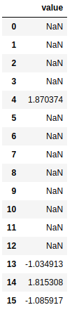

From this data we see that all of our data falls within 95% of our normal distribution of data and gives us no cause for concern.

Conclusions

We have successfully created a model and checked that we did not violate any of our assumptions we made in the previous post. We saw that our data was approximately normal, but did have some non-homogenous variance. Because we have a balanced data set we realized that our F-test would not be dramatically affected. We also tested our data for outliers and came to the conclusion that were none.