This post is the first of two posts to focus on how to perform an exploratory data analysis (EDA) of the experimental data set, create a hypothesis and perform an analysis of variance (ANOVA) on the hypothesis. The second part will focus on how to build a model and determine if the model is valid. My background is in nanotechnology so this post will focus on a simple experiment where the experimenter would like to test the differences in plasma power on deposition of a thin film on the surface of a silicon wafer. Values are made up and completely my own. All analysis will be performed in Python using the SciPy package and written in Jupyter notebooks.

Outline

• What is ANOVA
• Experimental Set-Up
• Exploratory Data Analysis
• Setting up data set in Python
• Degrees of Freedom
• Sum of Squares
• Mean Square Values
• F-Value and Testing our Hypothesis
• Conclusions

What is ANOVA?

Analysis of Variance is analyzing the variance between different treatments. The statistical test is called a one-way-ANOVA due to only one factor. When setting up an experiment, there will be different treatments or levels within that factor and then repeats within those treatments. ANOVA looks at how the data varies between different treatments (the between), within those treatments (the random error) and the total variation. The averages and sum of squares are calculated and then a ratio of the variances is computed.

The hypothesis of this experiment is that there will be no difference between the different treatments. Since we are comparing the ratio of the variance between treatments and variance within those treatments we can use F as our test statistic. This is very useful for investigating if the changes you make in an experiment are statistically significant and gives you and idea how to proceed with your next set of follow up experiments. We will then build a model using the effects model:

where $y_{i,j}$ is the $ij^{th}$ observation, $\mu_i$ is the mean of the $i$th treatment, $\tau_{i}$ is the treatment effect and $\epsilon_{ij}$ is the random error component which captures all the varability within the experiment. The random error includes, measurement error (measurement tool), differences between samples (e.g. surface slightly different), and any environmental errors. The $i$ classifies the treatment number, and the $j$ represents the sample within the treatment. The importance of this model is that it allows us to “predict” or explain the the individual components of our value, $y_{ij}$.

Formally our null hypothesis is:

and our alternative hypothesis is:

I will break down these ideas and explain in more depth as we compute this in Python.

Experimental Set Up

To begin, I created a fictional data set (as a .csv) where I am interested in seeing how my plasma settings affect my CVD growth rate. I set up a completely randomized experiment with 1 factor (plasma power) and 4 treatment levels of plasma power (8, 10, 12, 14 Watts) with four replicates. The first step is to load the fictional data set into pandas and view the data.

# Basic SciPy packages
import numpy as np
import pandas as pd

# Stats Packages
from scipy import stats

# Graphing packages
import matplotlib.pyplot as plt
import seaborn as sns
sns.set_style("whitegrid")
%matplotlib inline

cvd_dataset = pd.read_csv("CVD_Dataset_EDA_ANOVA.csv")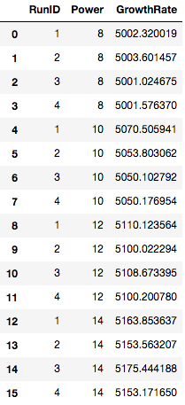

EDA-BoxPlot

The first steps in analyzing the data is to examine the data visually. This allows the experimenter to gauge how the treatments affects the growth rate. Let’s load the data and view it as a box chart.

sns.boxplot(x = "Power", y = "GrowthRate", data = cvd_dataset)
plt.xlabel(r"Power (W)")
plt.ylabel(r"Growth Rate ($\AA$ /min)")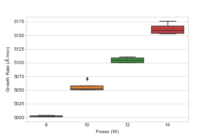

So what do we see? Visually, we can see that increasing the power leads to an increase in growth rate. Additionally, it appears that increasing power might contribute to increasing variability around the mean of each power setting but I can’t say for certain. So what is someone to do? Run the ANOVA on the data.

Setting up dataset in Python

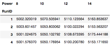
Before we can perform an ANOVA we need to re-arrange the data (especially visually for this post) so let’s pivot the dataset to view by “RunID” and “Power”.

cvd_pivot = cvd_dataset.pivot(index = 'RunID', 
                columns = 'Power', values = 'GrowthRate')
cvd_pivot

In the above table, we see that we have the different treatments in the columns and our repeat samples in the rows.

Degrees of Freedom

Next up, we need to determine the degrees of freedom. The degrees of freedom tells us how many independent moves the system can make. We will look at three different degrees of freedom, df between treatments, df within treatments(measurement error) and df total. We will call these dft, dfe, dftotal respectfully.

def degrees_of_freedom(df_pivot):
    ## Between samples is across the row
    ## Within samples is down the column
    n = df_pivot.count(axis=1) # Define number of replicates within treatment
    a = df_pivot.count() # Determine number of treatments
    n = n.iloc[0]
    a = a.iloc[0]
    
    TotalN = n*a # Total number of samples
    dft = a - 1 #dft is degrees of freedom between sample set
    dfe = TotalN - a #dfe is degrees of freedom within samples
    dftotal = TotalN-1 #dftotal is degrees of freedom total 
    return dft, dfe, dftotal, n, a 

And lets view these values:

dft, dfe, dftotal = degrees_of_freedom(cvd_pivot)

print("Degrees of freedom between treatments: {:d}".format(dft))
print("Degrees of freedom within treatments: {:d}".format(dfe))
print("Total degrees of freedom: {:d}".format(dftotal))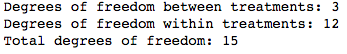

Sum of Squares

Now comes the heart of the ANOVA, calculating the sum of squares but first let’s define a few more things. First, $y_{i.}$ is the sum of the observations for treatment, $i$:

We can then find the average of the sums, $\bar{y}_{i.}/n$ which is

Finally the grand sum, $y_{..}$ is defined as:

and the grand average, $\bar{y}_{..}=y_{..}/N$

The first sum of squares to calculate is the sum of squares between treatments $SSTR$:

the sum of squares within treatments (error), $SSE$:

and the total sum of squares, $SST$:

Let’s convert these equations into a python function to quickly compute these equations for us.

def compute_sums(df_pivot):
    yi_sum = df_pivot.sum() # Compute sum under i-th treatment
    yi_avg = df_pivot.mean() # Compute average under i-th treatment 
    y_sum = yi_sum.sum() # Compute grand sum
    y_avg = yi_avg.mean() # Compute grand average
    return yi_sum, yi_avg, y_sum, y_avg

yi_sum, yi_avg, y_sum, y_avg = compute_sums(cvd_pivot) #retrieve respective sums by calling function

print(r"The sum under each Power (W) treatment is: {}".format(yi_sum))
print(r"The average under each Power (W) treatment is: {}".format(yi_avg))
print(r"The grand sum is: {:.2f}".format(y_sum))
print(r"The grand average is: {:.2f}".format(y_avg))    

def Sum_of_Squares(yi_avg, y_avg, df_pivot):
    SSTR = (yi_avg - y_avg)**2 #Calculate sum of squares between treatments
    SSTR = SSTR.sum()*n
    SSE = df_pivot.sub(yi_avg.values) ** 2 #Calculate sum of squares within treatments
    SSE = SSE.sum().sum()
    SST = SSTR + SSE # Total corrected sum of squares
    return SSTR, SSE, SST

SSTR, SSE, SST = Sum_of_Squares(yi_avg,y_avg, cvd_pivot)

print("Sum of Squares between treatments is: {:.2f}".format(SSTR))
print("Sum of Squares within treatments is: {:.2f}".format(SSE))
print("Total Sum of Squares is: {:.2f}".format(SST))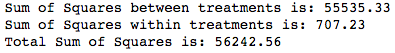

One immediate effect visible from computing the sum of squares is that the SSTR is much larger than the sum of squares within and tell us the treatments have a much larger effect than the within samples error has on the result.

Mean Square

To get to the F-Value we need to calculate the mean squares which is the sum of squares divided by their respective degrees of freedom.

def Mean_Squares(SSTR, SSE, dft, dfe):
    MSTR = SSTR/(dft) ## Mean Square between Treatments
    MSE = SSE/(dfe) ## Mean Square Error (within)
    return MSTR, MSE

MSTR, MSE = Mean_Squares(SSTR, SSE, dft, dfe)

print("Mean squares between treatments is: {:.2f}".format(MSTR))
print("Mean squares within treatments is: {:.2f}".format(MSE))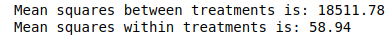

F-Value and Testing our Hypothesis

We have finally come to the F-Value. I will leave the theory behind it for another post, but this is where we can finally test our hypothesis.

Our null hypothesis is:

and our alternative hypothesis is:

We calculate our F-Value using:

We set our $\alpha = 0.05$ and can reject our $H_{0}$ if our $p \le 0.05$. We can compute our $$p from our F-Value using python.

F = MSTR/MSE #F-value
p = stats.f.sf(F, dft, dfe)

print("F-value is: {:.2f}".format(F))
print("p-value is: {:.3f}".format(p))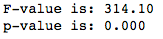

From this we see our p-value is $\le$ 0.05 so we can reject our null hypothesis and statistically say that our treatment means are different.

So that was really long an involved so lets check our answer using the built-in function.

from scipy import stats

f_val, p_val = stats.f_oneway(cvd_pivot[8], 
                cvd_pivot[10], cvd_pivot[12], cvd_pivot[14])  
print("F-value is: {:.2f}".format(f_val))
print("p-value is: {:.3f}".format(p_val))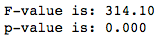

We can now report that our power setting greatly alters the average growth rate of our CVD film. We would report this as $F(3,12) = 314.10 \space p < 0.001$.

Conclusions

After performing the ANOVA, we can conclude that our different plasma levels are statistically different due to rejecting the null hypothesis. We could initially visualize this from our box plots, and see the sum of squares for the treatments were much greater than within treatments. We tested this by setting up a hypothesis that there was no difference and then using an using an F-test to test the hypothesis. Since the p-value for our F-test was much less than 0.05 we could conclude that there was a significant difference between treatments and could reject our null hypothesis.

So what do we do next and how is this useful for CVD or materials science? Well we can now develop a model and check our assumptions which will be discussed in Part II.